Examples¶

Here is a collection of grid examples and how to write them to GGD.

Example 1: Minimalistic unstructured grid example¶

In this example we will describe a simple unstructured grid (single time slice) consisting of one 2D object - surface to present the basic concepts behind GGD.

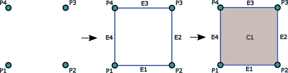
../_images/grid_structure_1.png — Grid consisting of one 2D object which is composed by 4 points / 4 edges / 1 2D cell.¶

Defining the grid¶

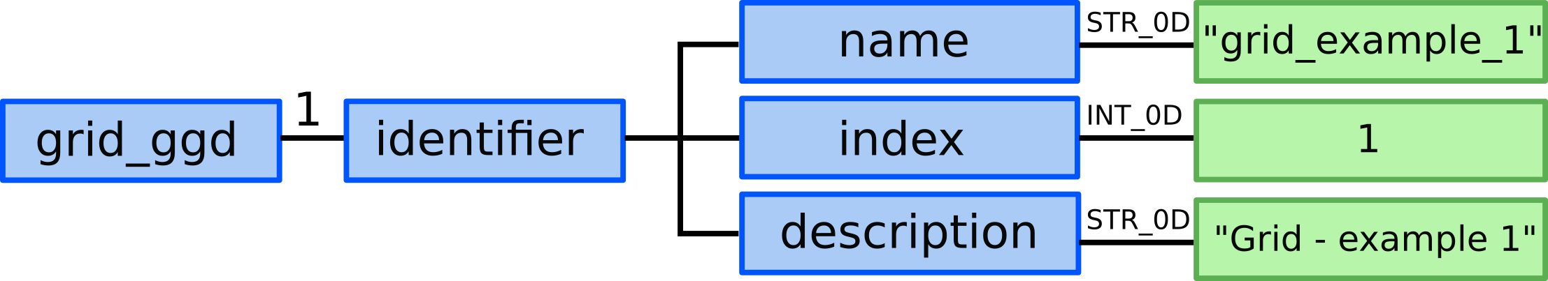
1.) We need to allocate one grid_ggd AOS (one time slice).

2.) In grid_ggd(1).identifier we define the grid name, index and description:

grid_ggd(1).identifier.name = "grid_example_1"
grid_ggd(1).identifier.index = 1
grid_ggd(1).identifier.description = "Grid - example 1"

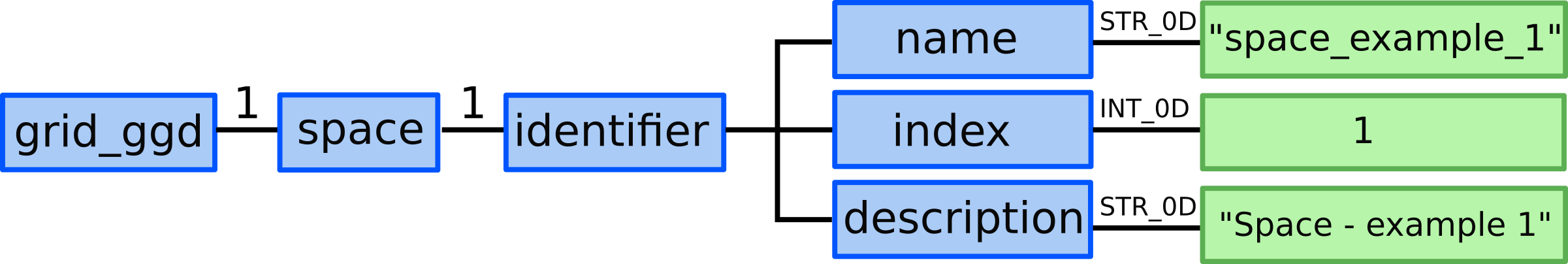
3.) We allocate one grid_ggd(1).space AOS.

4.) In grid_ggd(1).space(1).identifier node we define the space name, index and description:

grid_ggd(1).space(1).identifier.name = "space_example_1"
grid_ggd(1).space(1).identifier.index = 1
grid_ggd(1).space(1).identifier.description = "Space - example 1"

5.) In grid_ggd(1).space(1).geometry_type.index leaf we define standard geometry -> index 0

grid_ggd(1).space(1).geometry_type.index = 0

6.) In grid_ggd(1).space(1).coordinates_type leaf we define two coordinates following the coordinate_identifier this way defining 2D space. We define 1 and 2 meaning X and Y coordinates:

grid_ggd(1).space(1).coordinate_types = [1, 2]

7.) We allocate three grid_ggd(1).space(1).objects_per_dimension AOSs: for 0D objects - points, 1D objects - edges/lines, and 2D objects - surfaces/2D cells.

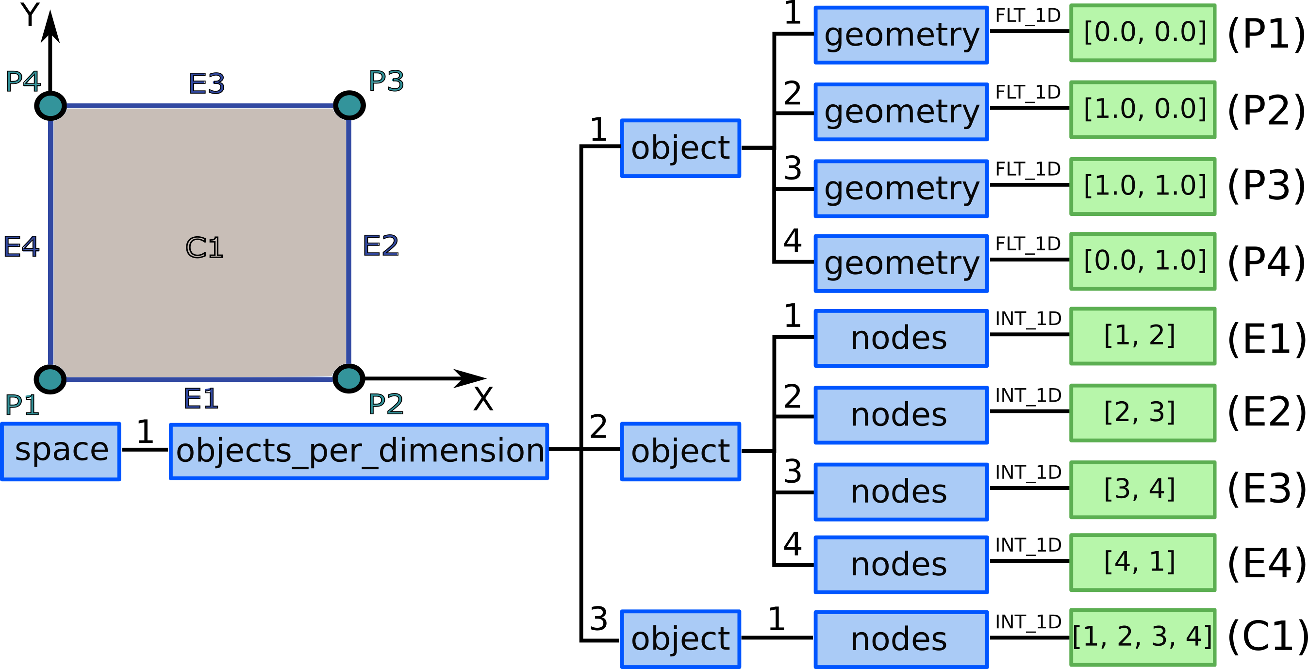
8.1) We allocate 4 ...objects_per_dimension(1).object AOS as our grid consists of 4 points.

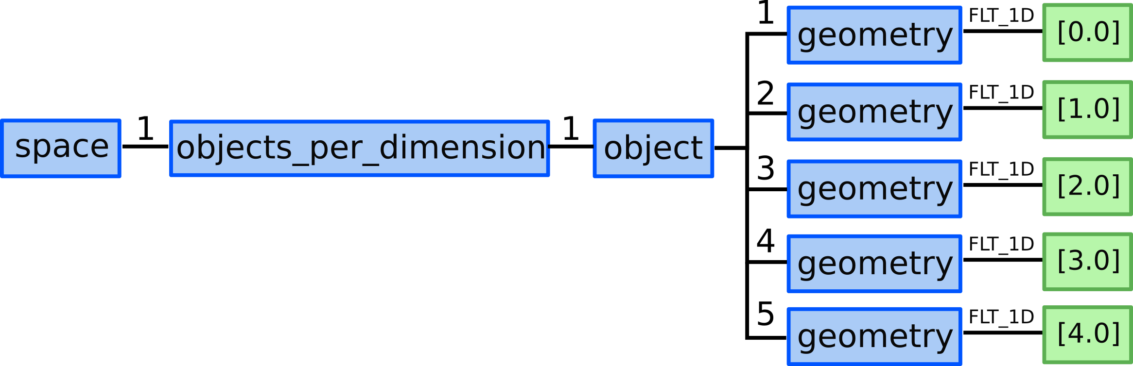
8.2) We define 4 points by defining their geometry (note that the coordinates are simplified according to the example):

...objects_per_dimension(1).object(1).geometry = [0.0, 0.0]
...objects_per_dimension(1).object(2).geometry = [1.0, 0.0]
...objects_per_dimension(1).object(3).geometry = [1.0, 1.0]
...objects_per_dimension(1).object(4).geometry = [0.0, 1.0]

9.1) We allocate 4 ...objects_per_dimension(2).object AOS as our grid consists of 4 lines.

9.2) We define 4 lines by defining nodes that compose each line (see figure Grid consisting of one 2D object which is composed by 4 points / 4 edges / 1 2D cell.):

...objects_per_dimension(2).object(1).nodes = [1, 2]
...objects_per_dimension(2).object(2).nodes = [2, 3]
...objects_per_dimension(2).object(3).nodes = [3, 4]
...objects_per_dimension(2).object(4).nodes = [4, 1]

10.1) We allocate 1 ...objects_per_dimension(3).object AOS as our grid consists of 1 quadrilateral cell.

10.2) We define 1 quadrilateral cell by defining 4 nodes that compose the quadrilateral (see figure Grid consisting of one 2D object which is composed by 4 points / 4 edges / 1 2D cell.):

...objects_per_dimension(3).object(1).nodes = [1, 2, 3, 4]

Now we have all grid objects in the domain defined.

Defining grid subsets¶

In our case we don’t have any specific grid subsets, however, we still need to define the grid subsets correlating to the 0D, 1D and 2D objects in the domain. This is due to Data Dictionary description, as physical quantities correlate directly to grid subsets and not to the grid itself.

The agreed grid subset labels can be found here: ggd_subset_identifier.

11.1) Allocate 3 grid_ggd(1).grid_subset AOSs (nodes, faces, 2D cells):

11.2) Define nodes grid subset. By definition nodes grid subset is composed by all 0D objects defined in this grid_ggd AOS so the element AOS can be left empty.

grid_ggd(1).grid_subset(1).dimension = 1
grid_ggd(1).grid_subset(1).identifier.name = "nodes"
grid_ggd(1).grid_subset(1).identifier.index = 1
grid_ggd(1).grid_subset(1).identifier.description = "All nodes in the domain"

11.3) Define faces grid subset. By definition faces grid subset is composed by all 0D objects defined in this grid_ggd AOS so the element AOS can be left empty.

grid_ggd(1).grid_subset(2).dimension = 2
grid_ggd(1).grid_subset(2).identifier.name = "faces"
grid_ggd(1).grid_subset(2).identifier.index = 2
grid_ggd(1).grid_subset(2).identifier.description = "All lines in the domain"

11.4) Define cells grid subset. By definition cells grid subset is composed by all 0D objects defined in this grid_ggd AOS so the element AOS can be left empty.

grid_ggd(1).grid_subset(3).dimension = 3
grid_ggd(1).grid_subset(3).identifier.name = "cells"
grid_ggd(1).grid_subset(3).identifier.index = 5
grid_ggd(1).grid_subset(3).identifier.description = "All 2D cells in the domain"

With this last step the grid description of our minimalistic unstructured grid example is finished.

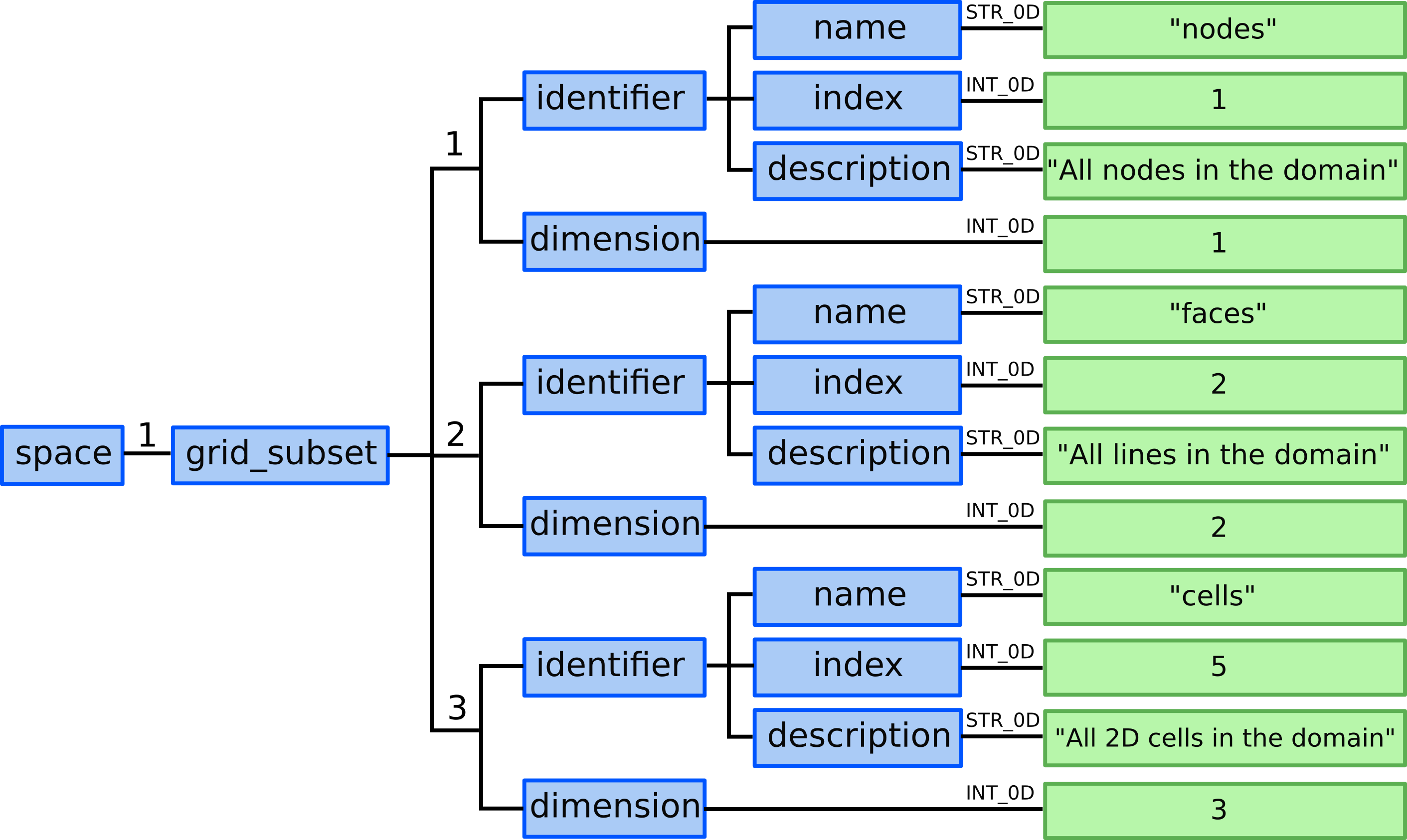
../_images/example_1_6.png — Defining the three base grid subsets - **nodes**, **faces** and **cells**. Note that the dimension ID doesn’t start with 0 as 0 values are in Data Dictionary reserved for **undefined indices**.¶

Defining physical quantities¶

Suppose that we have electron temperature and ion specie Ne+2 density quantities/values for single time slice at time 1.0ms that correlate to our 4 nodes and to our one 2D cell. Defining them in GGD is done in the next way:

12.) We need to allocate one ggd AOS (one time slice).

13.) We specify time of this time slice:

ggd(1).time = 1.0

Electron temperature¶

14.) We allocate two ggd(1).electrons.temperature AOS as in this case we have available electron temperature quantities for two grid subsets.

15.) In ggd(1).electrons.temperature(1) we define grid_index, grid_subset_index and values leafs.

grid_index and grid_subset_index are used to navigate to grid which has grid_ggd(:).identifier.index == grid_index and :grid_ggd(:).grid_subset(:).identifier.index == grid_subset_index. In this case it would navigate to our nodes grid subset.

ggd(1).electrons.temperature(1).grid_index = 1
ggd(1).electrons.temperature(1).grid_subset_index = 1
ggd(1).electrons.temperature(1).values = e.g. [1.1, 2.2, 3.3, 4.4] (one value per point)

16.) In ggd(1).electrons.temperature(2) we define grid_index, grid_subset_index and values leafs.

ggd(1).electrons.temperature(2).grid_index = 1
ggd(1).electrons.temperature(2).grid_subset_index = 2
ggd(1).electrons.temperature(2).values = e.g. [2.5] (one value per cell)

Ion density - specie Ne+2¶

17.) We allocate one ggd(1).ion AOS (as we have one ion specie).

18.) We define ion specie label:

ggd(1).ion(1).label = “Ne+”

19.) We allocate one ion state ggd(1).ion(1).state AOS as we have one state - Ne+2. Other states could be Ne+3 ,**Ne+4**, etc., however we don’t have those in this example.

20.) We allocate two ggd(1).ion(1).state(1).density AOS (for nodes and cells grid subsets).

21.) We define ion specie state label:

ggd(1).ion(1).label = “Ne+2”

22.) In ggd(1).ion(1).state(1).density(1) we define grid_index, grid_subset_index and values leafs.

ggd(1).ion(1).state(1).density(1).grid_index = 1
ggd(1).ion(1).state(1).density(1).grid_subset_index = 1
ggd(1).ion(1).state(1).density(1).values = e.g. [0.1, 0.2, 0.3, 0.4] (one value per point)

23.) In ggd(1).ion(1).state(1).density(2) we define grid_index, grid_subset_index and values leafs.

ggd(1).ion(1).state(1).density(2).grid_index = 1
ggd(1).ion(1).state(1).density(2).grid_subset_index = 2
ggd(1).ion(1).state(1).density(2).values = e.g. [0.3] (one value per cell)

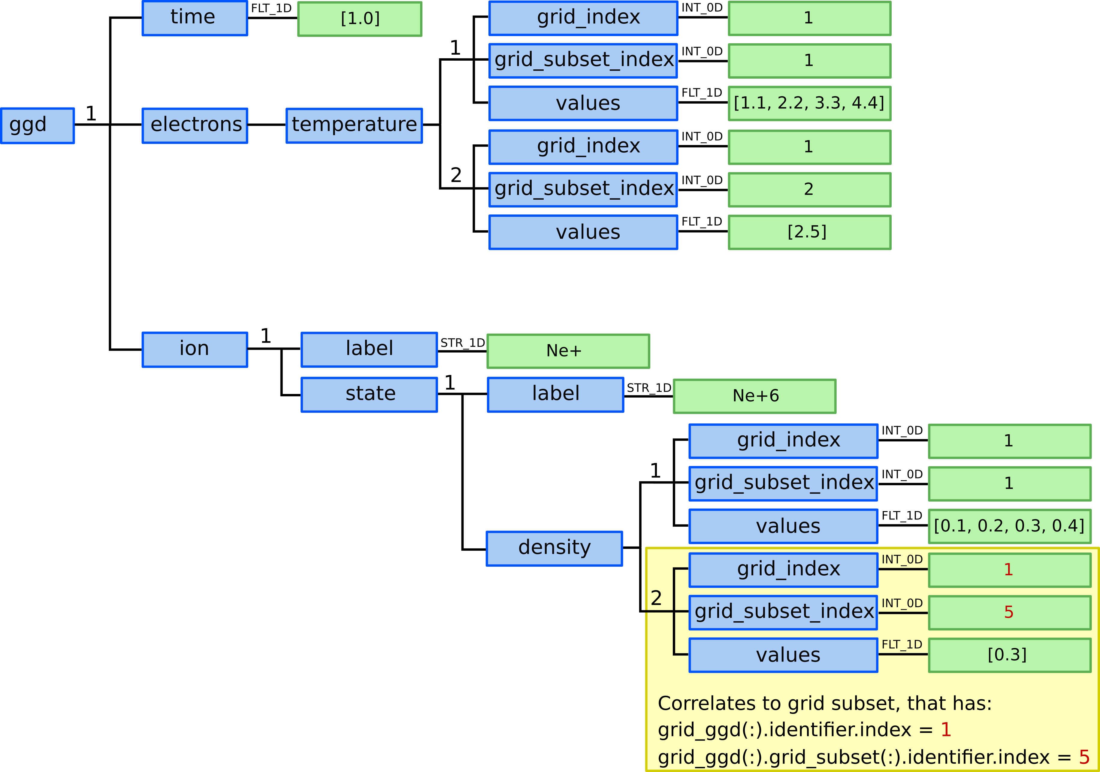
../_images/example_1_7.png — Defining physical quantities and their correlation to grid subsets.¶

Example 2: Minimalistic structured grid example¶

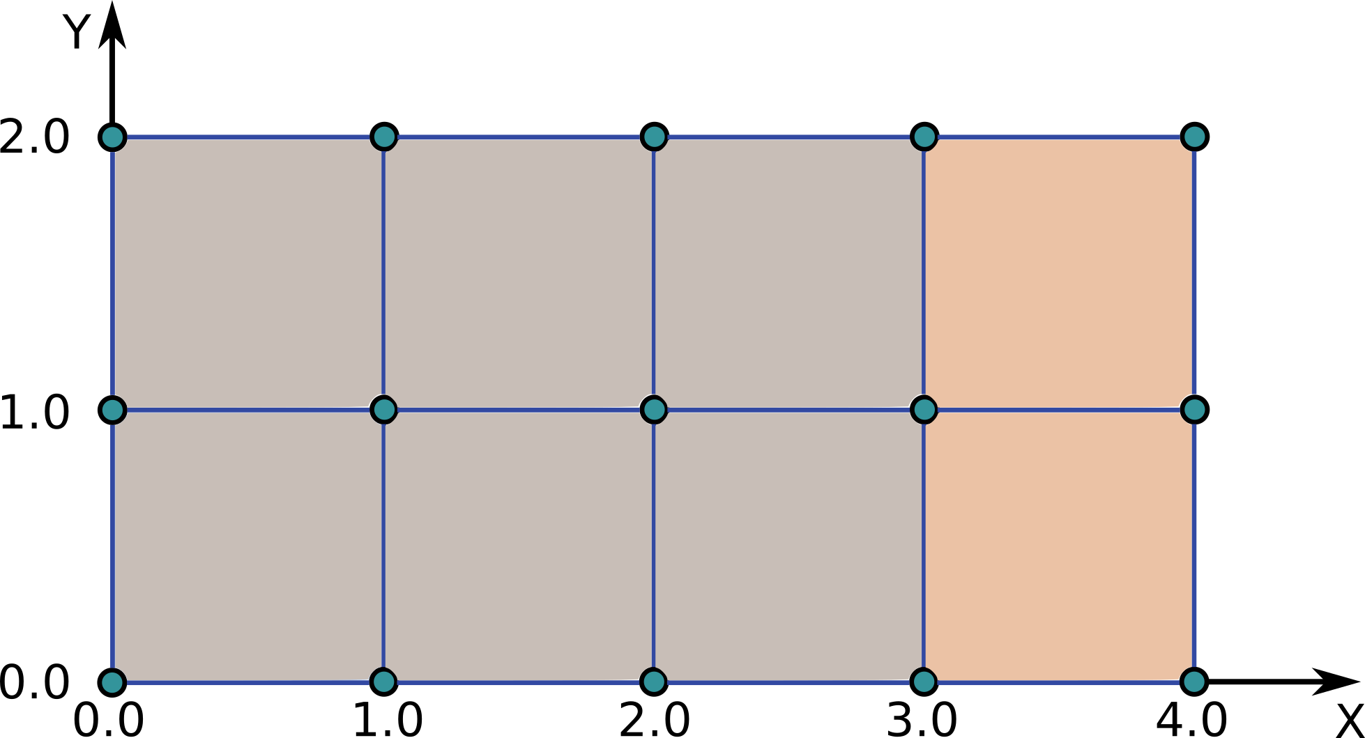
In this example we will describe a simple structured grid (two time slices) consisting of 5 points in X direction, and 3 points in Y direction to present the basic concepts behind GGD.

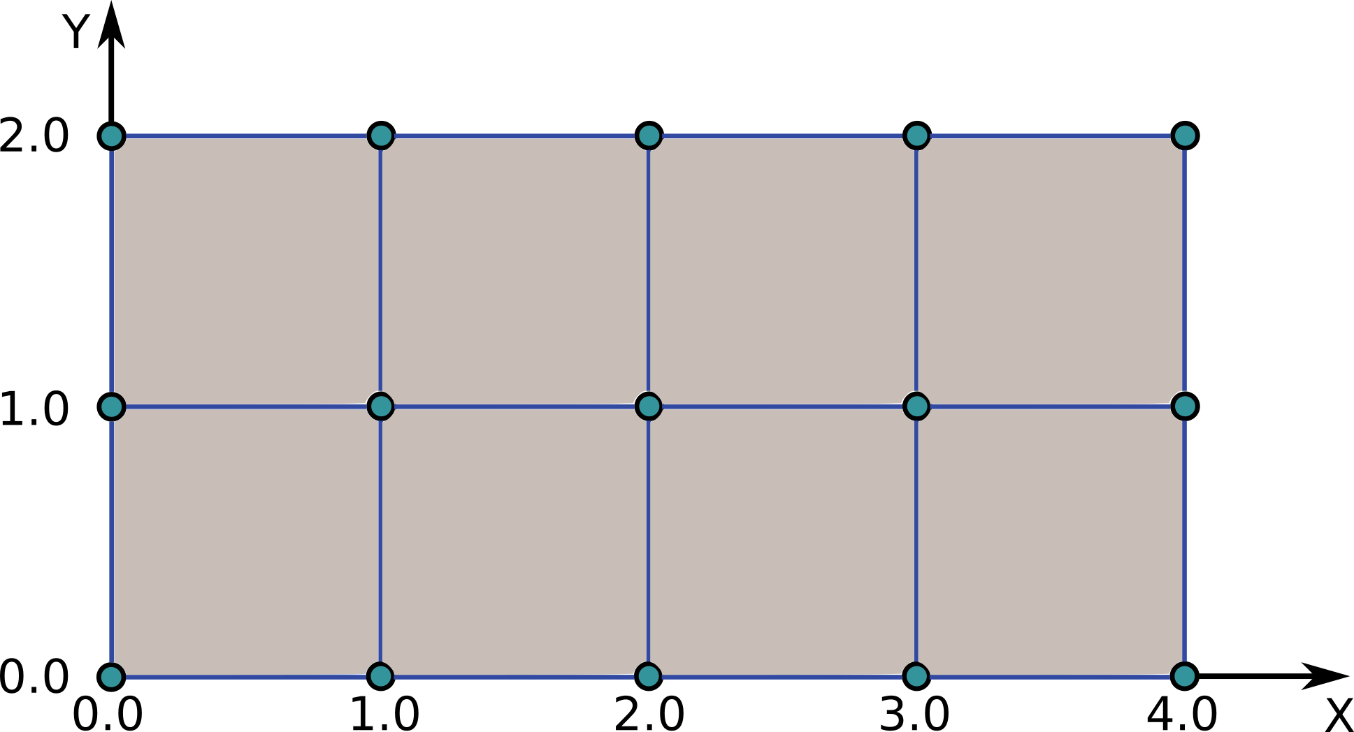
../_images/example_2_1.png — Grid consisting of consisting of 5 points in X direction, and 3 points in Y direction.¶

Defining the grid¶

1.) We need to allocate one grid_ggd AOS. Grid will remain static through the next time slice so we can define it only for one “time slice”.

2.) In grid_ggd(1).identifier we define the grid name, index and description:

grid_ggd(1).identifier.name = "grid_example_2"
grid_ggd(1).identifier.index = 1
grid_ggd(1).identifier.description = "Grid - example 2"

3.) We allocate two grid_ggd(1).space AOSs. One for X direction and the second for Y direction.

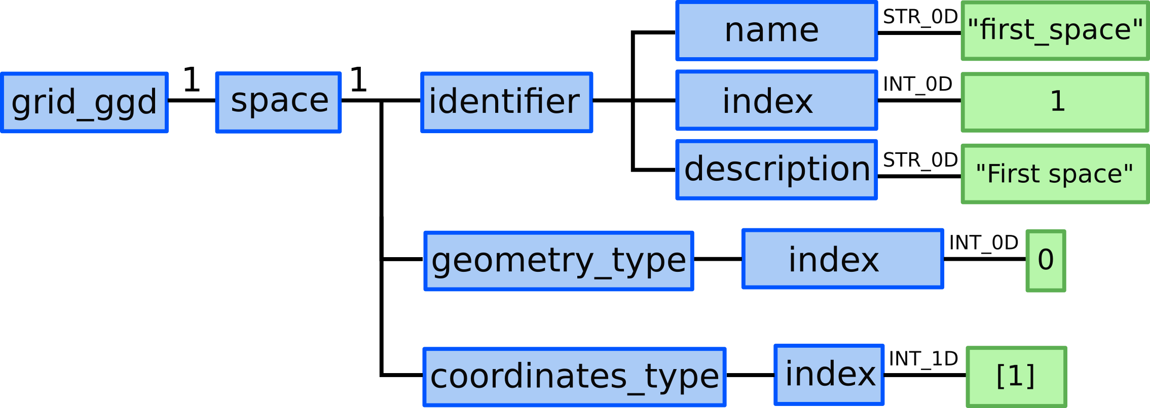
Space 1 - X direction¶

4.) In grid_ggd(1).space(1).identifier node we define the space name, index and description:

grid_ggd(1).space(1).identifier.name = "first_space"
grid_ggd(1).space(1).identifier.index = 1
grid_ggd(1).space(1).identifier.description = "First Space"

5.) In grid_ggd(1).space(1).geometry_type.index leaf we define standard geometry -> index 0.

6.) In grid_ggd(1).space(1).coordinates_type leaf we define one coordinate following the coordinate_identifier this way defining 1D space. We define 1 meaning X coordinate:

7.) We allocate one grid_ggd(1).space(1).objects_per_dimension AOSs: for 0D objects - points in X direction.

8.1) We allocate 5 ...objects_per_dimension(1).object AOS as our structured grid consists of 5 points in X direction.

8.2) We define 5 points by defining their geometry:

...objects_per_dimension(1).object(1).geometry = [0.0]
...objects_per_dimension(1).object(2).geometry = [1.0]
...objects_per_dimension(1).object(3).geometry = [2.0]
...objects_per_dimension(1).object(4).geometry = [3.0]
...objects_per_dimension(1).object(5).geometry = [4.0]

Space 2 - Y direction¶

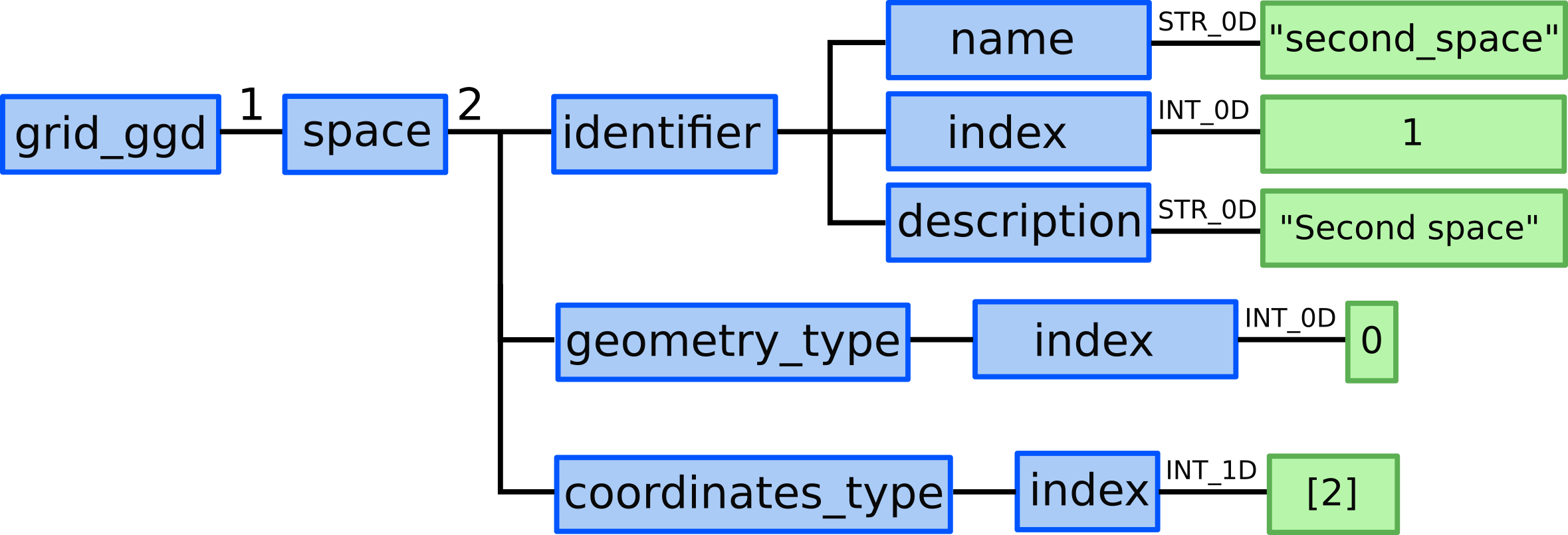
9.) In grid_ggd(1).space(2).identifier node we define the space name, index and description:

grid_ggd(1).space(2).identifier.name = "second_space"
grid_ggd(1).space(2).identifier.index = 1
grid_ggd(1).space(2).identifier.description = "Second Space"

10.) In grid_ggd(1).space(2).geometry_type.index leaf we define standard geometry -> index 0

11.) In grid_ggd(1).space(2).coordinates_type leaf we define one coordinate following the coordinate_identifier this way defining 1D space. We define 2 meaning Y coordinate:

12.) We allocate one grid_ggd(1).space(2).objects_per_dimension AOSs: for 0D objects - points in X direction.

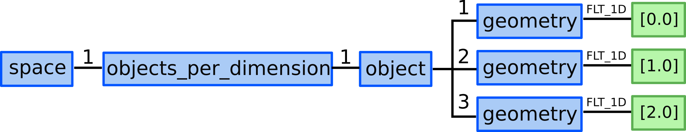
13.1) We allocate 3 ...objects_per_dimension(1).object AOS as our structured grid consists of 3 points in Y direction.

13.2) We define 5 points by defining their geometry:

...objects_per_dimension(1).object(1).geometry = [0.0]
...objects_per_dimension(1).object(2).geometry = [1.0]
...objects_per_dimension(1).object(3).geometry = [2.0]

Defining grid subsets¶

We need to define the grid subsets correlating to the 0D, 1D and 2D objects in the domain. This is due to Data Dictionary description, as physical quantities correlate directly to grid subsets and to the grid itself.

The agreed grid subset labels can be found here: ggd_subset_identifier.

14.2) Allocate 3 grid_subsets (nodes, faces, 2D cells):

Base grid subsets¶

15.2) Define nodes grid subset. By definition nodes grid subset is composed by all 0D objects defined in this grid_ggd AOS so the element AOS can be left empty.

grid_ggd(1).grid_subset(1).dimension = 1
grid_ggd(1).grid_subset(1).identifier.name = "nodes"
grid_ggd(1).grid_subset(1).identifier.index = 1
grid_ggd(1).grid_subset(1).identifier.description = "All nodes in the domain"

15.3) Define faces grid subset. By definition faces grid subset is composed by all 0D objects defined in this grid_ggd AOS so the element AOS can be left empty.

grid_ggd(1).grid_subset(2).dimension = 2
grid_ggd(1).grid_subset(2).identifier.name = "faces"
grid_ggd(1).grid_subset(2).identifier.index = 2
grid_ggd(1).grid_subset(2).identifier.description = "All lines in the domain"

15.4) Define cells grid subset. By definition cells grid subset is composed by all 0D objects defined in this grid_ggd AOS so the element AOS can be left empty.

grid_ggd(1).grid_subset(3).dimension = 3
grid_ggd(1).grid_subset(3).identifier.name = "cells"
grid_ggd(1).grid_subset(3).identifier.index = 3
grid_ggd(1).grid_subset(3).identifier.description = "All 2D cells in the domain"

Defining physical quantities¶

Suppose that we have electron temperature quantities/values for two time slices at times 1.0ms and 2.0ms that correlate to our 15 points (we assume that we don’t have any data for 2D cells). Defining them in GGD is done in the next way:

16.) We need to allocate two ggd AOS (two time slices).

17.) We specify time value for both time slices:

ggd(1).time = 1.0
ggd(2).time = 2.0

Electron temperature - First time slice¶

18.) We allocate one ggd(1).electrons.temperature AOS as in this case we have available electron temperature quantities for one grid subset.

19.) In ggd(1).electrons.temperature(1) we define grid_index, grid_subset_index and values leafs.

ggd(1).electrons.temperature(1).grid_index = 1
ggd(1).electrons.temperature(1).grid_subset_index = 1
ggd(1).electrons.temperature(1).values = e.g. [1.1, 2.2, …, 15.15] (one value per point, 15 values)

Electron temperature - Second time slice¶

20.) We allocate one ggd(1).electrons.temperature AOS as in this case we have available electron temperature quantities for one grid subset.

21.) In ggd(1).electrons.temperature(1) we define grid_index, grid_subset_index and values leafs.

ggd(2).electrons.temperature(1).grid_index = 1
ggd(2).electrons.temperature(1).grid_subset_index = 1
ggd(2).electrons.temperature(1).values = e.g. [2.2, 3.3, …, 16.16] (one value per point, 15 values)

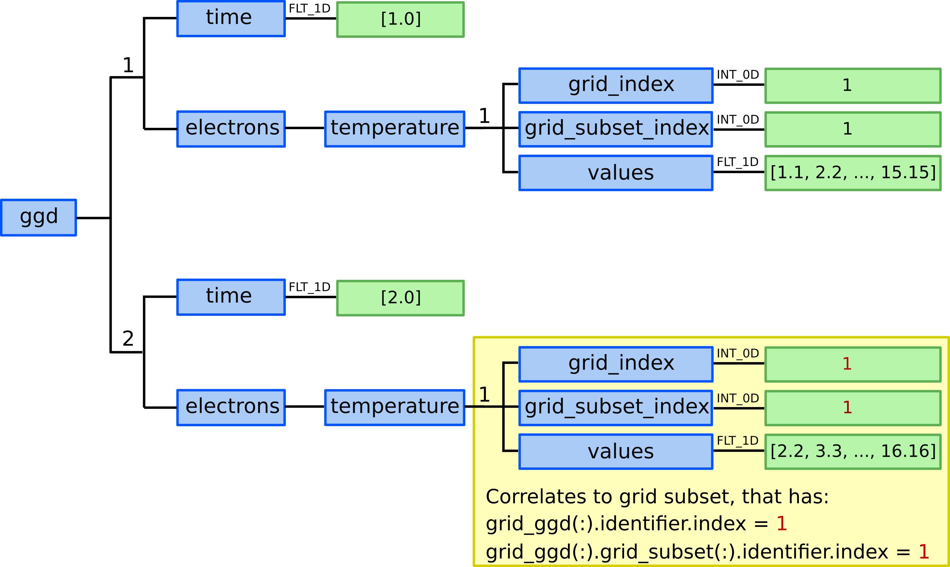
../_images/example_2_9.png — Defining electron temperature data fields for two time slices.¶

Example 3: Structured grid subset example¶

Following the Example 2: Minimalistic structured grid example, lets assume that the two right-most 2D cells represent our outer divertor grid subset, just for purposes to explain the grid subset concepts when dealing with structured grids.

Outer divertor grid subset¶

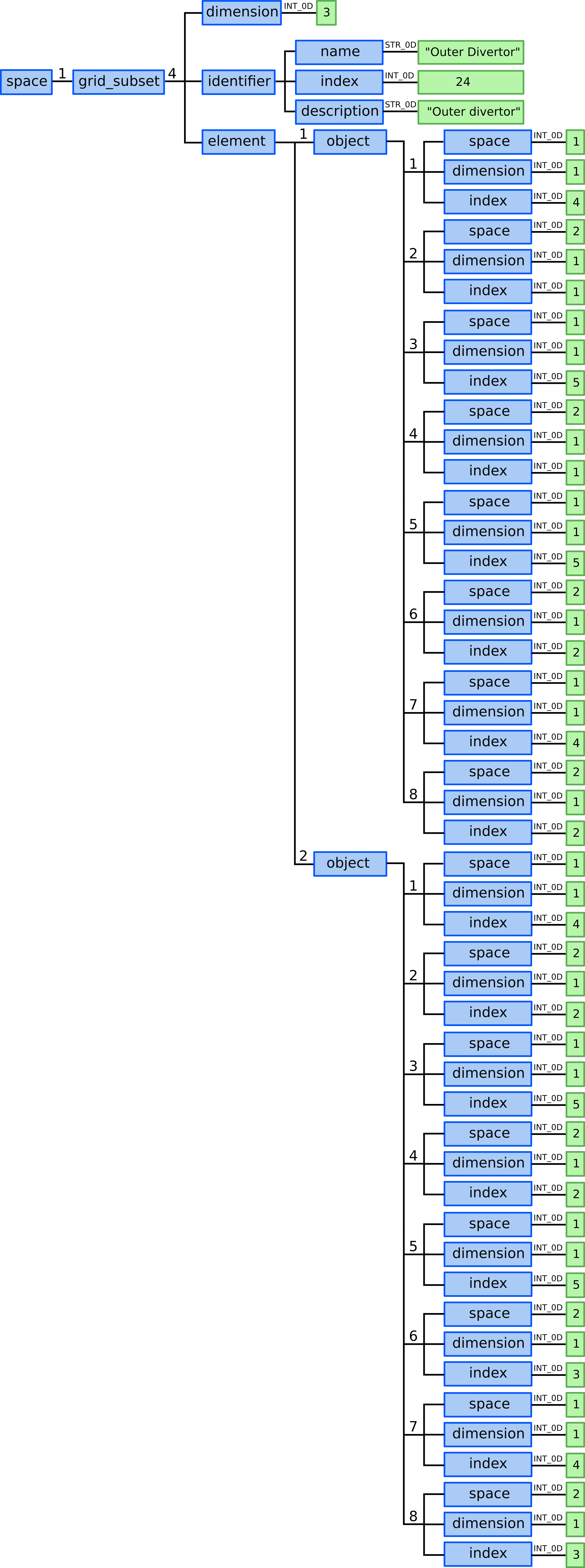
Our 4-th grid subset represents outer divertor region (just for explanation purposes), as seen in the figure below.

Now we need to define the elements which compose this grid subset. In this case, the elemets are 2D cells, and those 2D cells are composed by objects, in this case points defined on 1D spaces. So we will have 2 elements, each composed by 2x4 points which are defined on 1D spaces.

1.) Describe outer divertor grid subset. By grid subset identifiers definition (see ggd_subset_identifier) outer divertor is defined by index 24.

grid_ggd(1).grid_subset(4).dimension = 3
grid_ggd(1).grid_subset(4).identifier.name = "outer_divertor"
grid_ggd(1).grid_subset(4).identifier.index = 24
grid_ggd(1).grid_subset(4).identifier.description = "Outer Divertor"

2.) Allocate 2 element AOS and for each element AOS 8 object AOS.

3.1) Defining first element - 2D cell based on 4 points each defined using 1D spaces. The space, dimension and index indices are used to navigate through grid_ggd(1).space(space_index).objects_per_dimension(dimension_index).object(index):

First point:

grid_ggd(1).grid_subset(4).element(1).object(1).space = 1
grid_ggd(1).grid_subset(4).element(1).object(1).dimension = 1
grid_ggd(1).grid_subset(4).element(1).object(1).index = 4
grid_ggd(1).grid_subset(4).element(1).object(2).space = 2
grid_ggd(1).grid_subset(4).element(1).object(2).dimension = 1
grid_ggd(1).grid_subset(4).element(1).object(2).index = 1

Second point:

grid_ggd(1).grid_subset(4).element(1).object(3).space = 1
grid_ggd(1).grid_subset(4).element(1).object(3).dimension = 1
grid_ggd(1).grid_subset(4).element(1).object(3).index = 5
grid_ggd(1).grid_subset(4).element(1).object(4).space = 2
grid_ggd(1).grid_subset(4).element(1).object(4).dimension = 1
grid_ggd(1).grid_subset(4).element(1).object(4).index = 1

Third point:

grid_ggd(1).grid_subset(4).element(1).object(5).space = 1
grid_ggd(1).grid_subset(4).element(1).object(5).dimension = 1
grid_ggd(1).grid_subset(4).element(1).object(5).index = 5
grid_ggd(1).grid_subset(4).element(1).object(6).space = 2
grid_ggd(1).grid_subset(4).element(1).object(6).dimension = 1
grid_ggd(1).grid_subset(4).element(1).object(6).index = 2

Fourth point:

grid_ggd(1).grid_subset(4).element(1).object(7).space = 1
grid_ggd(1).grid_subset(4).element(1).object(7).dimension = 1
grid_ggd(1).grid_subset(4).element(1).object(7).index = 4
grid_ggd(1).grid_subset(4).element(1).object(8).space = 2
grid_ggd(1).grid_subset(4).element(1).object(8).dimension = 1
grid_ggd(1).grid_subset(4).element(1).object(8).index = 2

3.2) Defining second element - 2D cell based on 4 points each defined using 1D spaces:

First point:

grid_ggd(1).grid_subset(4).element(2).object(1).space = 1
grid_ggd(1).grid_subset(4).element(2).object(1).dimension = 1
grid_ggd(1).grid_subset(4).element(2).object(1).index = 4
grid_ggd(1).grid_subset(4).element(2).object(2).space = 2
grid_ggd(1).grid_subset(4).element(2).object(2).dimension = 1
grid_ggd(1).grid_subset(4).element(2).object(2).index = 2

Second point:

grid_ggd(1).grid_subset(4).element(2).object(3).space = 1
grid_ggd(1).grid_subset(4).element(2).object(3).dimension = 1
grid_ggd(1).grid_subset(4).element(2).object(3).index = 5
grid_ggd(1).grid_subset(4).element(2).object(4).space = 2
grid_ggd(1).grid_subset(4).element(2).object(4).dimension = 1
grid_ggd(1).grid_subset(4).element(2).object(4).index = 2

Third point:

grid_ggd(1).grid_subset(4).element(2).object(5).space = 1
grid_ggd(1).grid_subset(4).element(2).object(5).dimension = 1
grid_ggd(1).grid_subset(4).element(2).object(5).index = 5
grid_ggd(1).grid_subset(4).element(2).object(6).space = 2
grid_ggd(1).grid_subset(4).element(2).object(6).dimension = 1
grid_ggd(1).grid_subset(4).element(2).object(6).index = 3

Fourth point:

grid_ggd(1).grid_subset(4).element(2).object(7).space = 1
grid_ggd(1).grid_subset(4).element(2).object(7).dimension = 1
grid_ggd(1).grid_subset(4).element(2).object(7).index = 4
grid_ggd(1).grid_subset(4).element(2).object(8).space = 2
grid_ggd(1).grid_subset(4).element(2).object(8).dimension = 1
grid_ggd(1).grid_subset(4).element(2).object(8).index = 3

This way our grid subset outer divertor is defined.

Example 4: Unstructured grid subsets example¶

In this example we will describe unstructured grid (two time slices) in [R, Z] space consisting of

20 points (0D objects)
31 edges/lines (1D objects), and
12 surfaces/2D cells (2D objects).

This grid will contains 6 grid subsets, 3 base ones and four additional ones, according to ggd_subset_identifier:

nodes (all nodes in the domain),
faces (all lines/edges in the domain),
cells (all surfaces/2D cells in the domain),
x_aligned_faces (all X aligned lines),
y_aligned_faces (all Y aligned lines),
outer_divertor (marked with green quadrilaterals)

Note

In this example outer_divertor grid subset won’t represent the actual outer divertor region. It is only to give an insight how to represent grid subsets in the GGD.

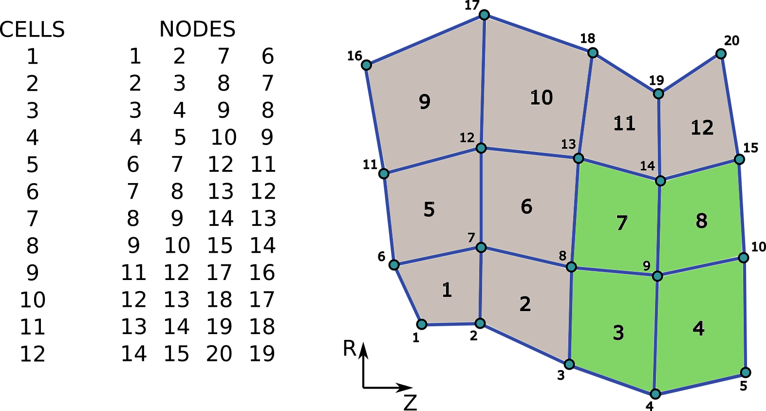
../_images/example_3_1.png — Unstructured grid used in this example and **connectivity array** for 2D objects - quadrilateral cells. Assumed grid subset “outer_divertor” is marked by green quadrilaterals.¶

Defining the grid¶

1.) We need to allocate one grid_ggd AOS (one AOS as we assume that grid does not change with time).

2.) In grid_ggd(1).identifier we define the grid name, index and description:

grid_ggd(1).identifier.name = "grid_example_4"
grid_ggd(1).identifier.index = 1
grid_ggd(1).identifier.description = "Grid - example 4"

3.) We allocate one grid_ggd(1).space AOS.

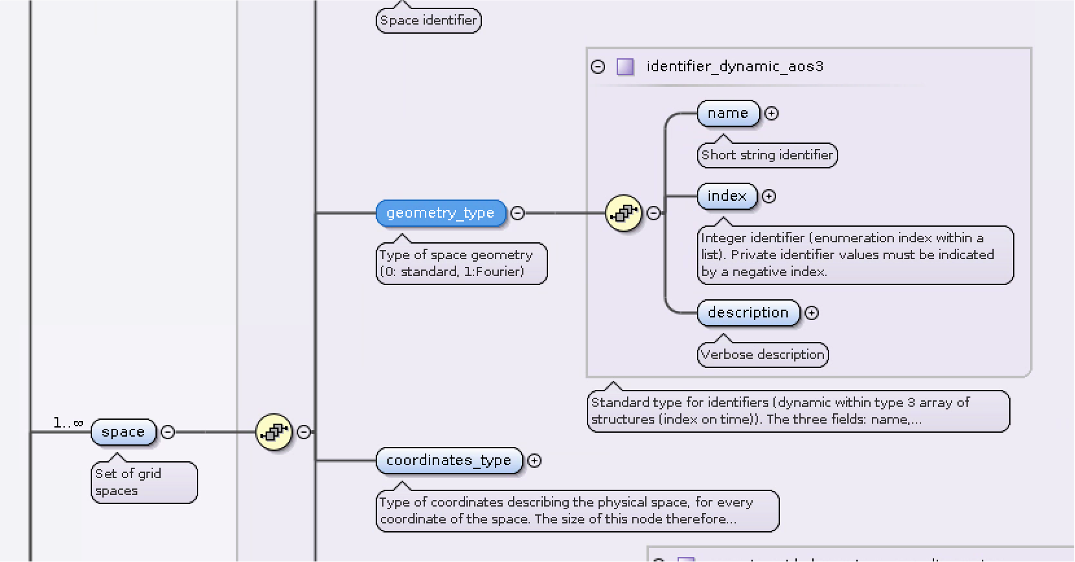
4.) In grid_ggd(1).space(1).identifier node we define the space name, index and description:

grid_ggd(1).space(1).identifier.name = "space_example_4"
grid_ggd(1).space(1).identifier.index = 1
grid_ggd(1).space(1).identifier.description = "Space - example 4"

5.) In grid_ggd(1).space(1).geometry_type.index leaf we define standard geometry -> index 0

grid_ggd(1).space(1).geometry_type.index = 0

6.) In grid_ggd(1).space(1).coordinates_type leaf we define two coordinates following the coordinate_identifier this way defining 2D space. We define 4 and 3 meaning R and Z coordinates according to coordinate_identifier:

grid_ggd(1).space(1).coordinate_types = [4, 3]

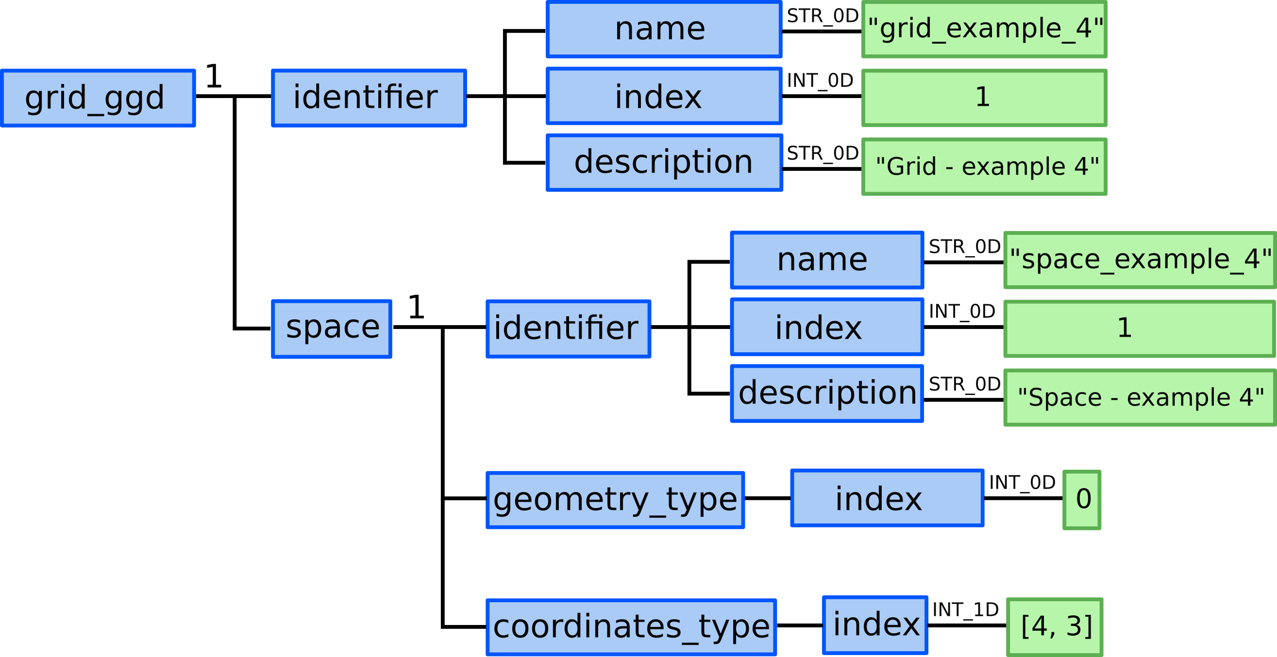
../_images/example_3_2.png — Representation of defining **grid** and **space** identifier name, index, and description; and space geometry_type and coordinates_type in GGD.¶

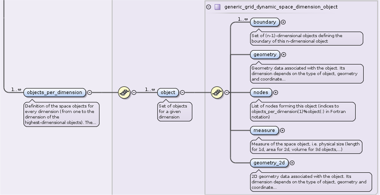
7.) We allocate three grid_ggd(1).space(1).objects_per_dimension AOSs: for 0D objects - points, 1D objects - edges/lines, and 2D objects - surfaces/2D cells.

8.1) We allocate 20 ...objects_per_dimension(1).object AOS as our grid consists of 20 points.

8.2) We define 20 points by defining their geometry (note that the coordinates are simplified and marked by \({r}\) and \({z}\) symbols instead of values according to the example):

...objects_per_dimension(1).object(1).geometry = [r_1, z_1]
...objects_per_dimension(1).object(2).geometry = [r_2, z_2]
...objects_per_dimension(1).object(3).geometry = [r_3, z_3]
…
...objects_per_dimension(1).object(20).geometry = [r_20, z_20]

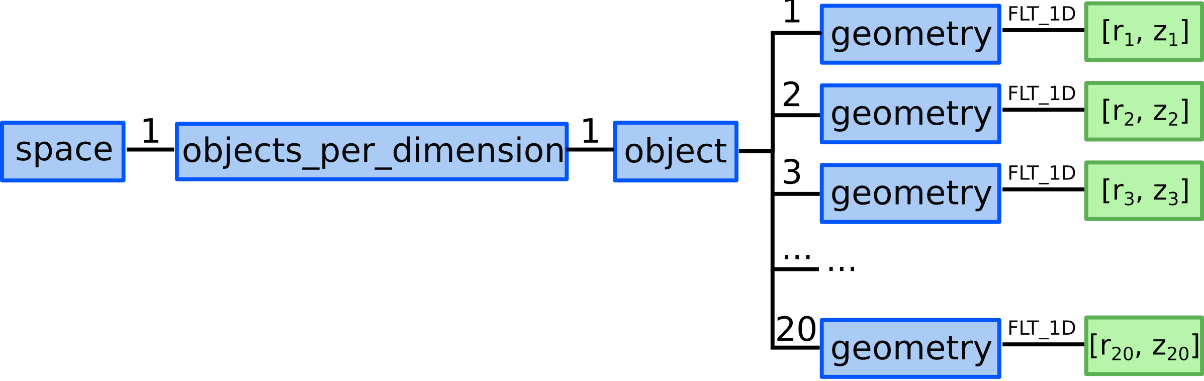
../_images/example_3_3.png — Representation of defining all 0D objects/points/nodes in the domain with GGD.¶

9.1) We allocate 31 ...objects_per_dimension(2).object AOS as our grid consists of 31 lines.

9.2) We define 31 lines by defining nodes that compose each line. First we define the “x-aligned (r-aligned)” lines and then the “y-aligned (z-aligned” lines.

...objects_per_dimension(2).object(1).nodes = [1, 2]
...objects_per_dimension(2).object(2).nodes = [2, 3]
...objects_per_dimension(2).object(3).nodes = [3, 4]
...objects_per_dimension(2).object(4).nodes = [4, 5]
...objects_per_dimension(2).object(5).nodes = [6, 7]
...objects_per_dimension(2).object(6).nodes = [7, 8]
...objects_per_dimension(2).object(7).nodes = [8, 9]
...objects_per_dimension(2).object(8).nodes = [9, 10]
...objects_per_dimension(2).object(9).nodes = [11, 12]
...objects_per_dimension(2).object(10).nodes = [12, 13]
...objects_per_dimension(2).object(11).nodes = [13, 14]
...objects_per_dimension(2).object(12).nodes = [14, 15]
...objects_per_dimension(2).object(13).nodes = [16, 17]
...objects_per_dimension(2).object(14).nodes = [17, 18]
...objects_per_dimension(2).object(15).nodes = [18, 19]
...objects_per_dimension(2).object(16).nodes = [19, 20]
...objects_per_dimension(2).object(17).nodes = [1, 6]
...objects_per_dimension(2).object(18).nodes = [6, 11]
...objects_per_dimension(2).object(19).nodes = [11, 16]
...objects_per_dimension(2).object(20).nodes = [2, 7]
...objects_per_dimension(2).object(21).nodes = [7, 12]
...objects_per_dimension(2).object(22).nodes = [12, 17]
...objects_per_dimension(2).object(23).nodes = [3, 8]
...objects_per_dimension(2).object(24).nodes = [8, 13]
...objects_per_dimension(2).object(25).nodes = [13, 18]
...objects_per_dimension(2).object(26).nodes = [4, 9]
...objects_per_dimension(2).object(27).nodes = [9, 14]
...objects_per_dimension(2).object(28).nodes = [14, 19]
...objects_per_dimension(2).object(29).nodes = [5, 10]
...objects_per_dimension(2).object(30).nodes = [10, 15]
...objects_per_dimension(2).object(31).nodes = [15, 20]

Note

The ...objects_per_dimension(2).object(:).measure could be filled with the line length, however we don’t need that information here.

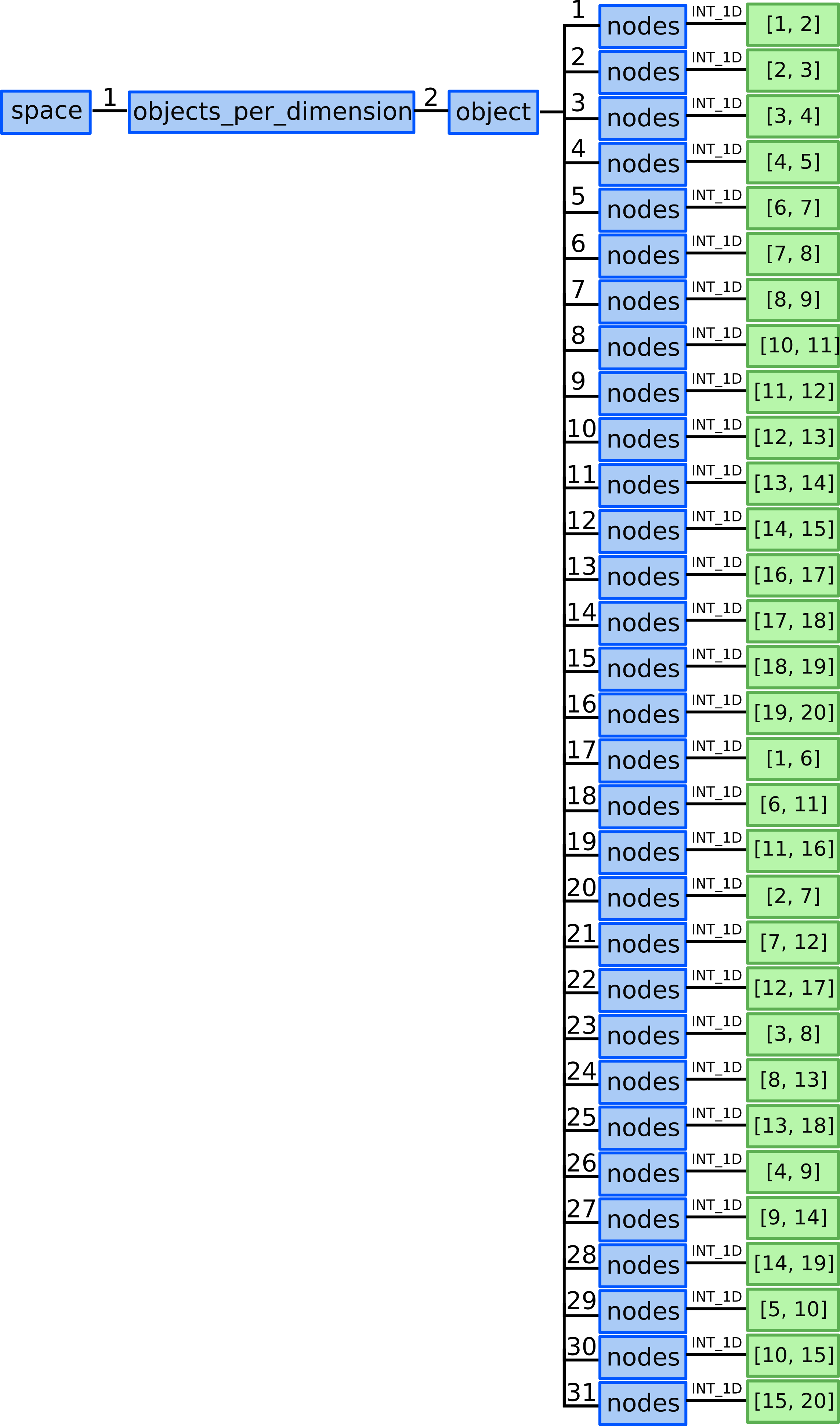
../_images/example_3_4.png — Representation of defining all 1D objects/lines in the domain with GGD.¶

10.1) We allocate 12 ...objects_per_dimension(3).object AOS as our grid consists of 12 quadrilateral cells.

10.2) We define connectivity array for 2D objects - 12 quads by defining nodes that compose each quad element.

...objects_per_dimension(3).object(1).nodes = [1, 2, 7, 6]
...objects_per_dimension(3).object(2).nodes = [2, 3, 8, 7]
...objects_per_dimension(3).object(3).nodes = [3, 4, 9, 8]
...objects_per_dimension(3).object(4).nodes = [4, 5, 10, 9]
...objects_per_dimension(3).object(5).nodes = [6, 7, 12, 11]
...objects_per_dimension(3).object(6).nodes = [7, 8, 13, 12]
...objects_per_dimension(3).object(7).nodes = [8, 9, 14, 13]
...objects_per_dimension(3).object(8).nodes = [9, 10, 15, 14]
...objects_per_dimension(3).object(9).nodes = [11, 12, 17, 16]
...objects_per_dimension(3).object(10).nodes = [12, 13, 18, 17]
...objects_per_dimension(3).object(11).nodes = [13, 14, 19, 18]
...objects_per_dimension(3).object(12).nodes = [14, 15, 20, 19]

Note

The ...objects_per_dimension(3).object(:).measure could be filled with the quad surface area, however we don’t need that information here.

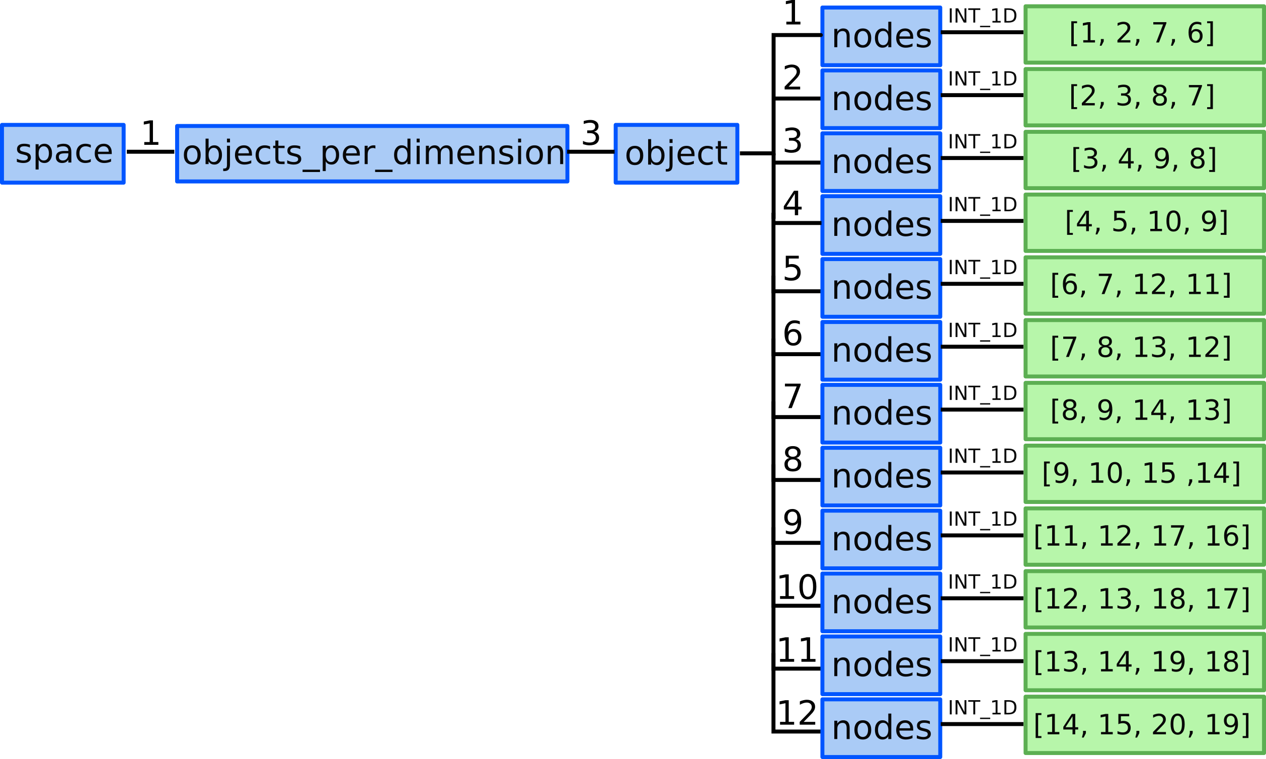
../_images/example_3_5.png — Representation of defining all 2D objects/quads in the domain with GGD.¶

Defining grid subsets¶

First we need to define the grid subsets correlating to the 0D, 1D and 2D objects in the domain. This is due to Data Dictionary description, as physical quantities (data fields) correlate directly to grid subsets and not to the grid itself.

Second, we will define 3 more grid subsets: x_aligned_faces, y_aligned_faces, and our “outer divertor” grid subset, giving us a total of 6 grid subsets.

The agreed grid subset labels can be found here: ggd_subset_identifier.

Allocate 6 grid_ggd(1).grid_subset AOSs:

12.1) Define nodes grid subset. By definition nodes grid subset is composed by all 0D objects defined in this grid_ggd AOS so the element AOS can be left empty.

grid_ggd(1).grid_subset(1).dimension = 1
grid_ggd(1).grid_subset(1).identifier.name = "nodes"
grid_ggd(1).grid_subset(1).identifier.index = 1
grid_ggd(1).grid_subset(1).identifier.description = "All nodes in the domain"

12.2) Define faces grid subset. By definition faces grid subset is composed by all 0D objects defined in this grid_ggd AOS so the element AOS can be left empty.

grid_ggd(1).grid_subset(2).dimension = 2
grid_ggd(1).grid_subset(2).identifier.name = "faces"
grid_ggd(1).grid_subset(2).identifier.index = 2
grid_ggd(1).grid_subset(2).identifier.description = "All lines in the domain"

12.3) Define cells grid subset. By definition cells grid subset is composed by all 0D objects defined in this grid_ggd AOS so the element AOS can be left empty.

grid_ggd(1).grid_subset(3).dimension = 3
grid_ggd(1).grid_subset(3).identifier.name = "cells"
grid_ggd(1).grid_subset(3).identifier.index = 3
grid_ggd(1).grid_subset(3).identifier.description = "All 2D cells in the domain"

12.3) Define x_alignes_faces grid subset. Here we need to define 16 elements each composed by single 1D object - face. Other option could be to define 16 elements each composed by two 0D objects - points, however we already have the lines defined in objects_per_dimension(2) so this is not necessary.

grid_ggd(1).grid_subset(4).dimension = 2
grid_ggd(1).grid_subset(4).identifier.name = "x_aligned_faces"
grid_ggd(1).grid_subset(4).identifier.index = 3
grid_ggd(1).grid_subset(4).identifier.description = "X aligned faces"
grid_ggd(1).grid_subset(4).element(1).object(1).space = 1
grid_ggd(1).grid_subset(4).element(1).object(1).dimension = 2
grid_ggd(1).grid_subset(4).element(1).object(1).index = 1
grid_ggd(1).grid_subset(4).element(2).object(1).space = 1
grid_ggd(1).grid_subset(4).element(2).object(1).dimension = 2
grid_ggd(1).grid_subset(4).element(2).object(1).index = 2

In this case all object AOSs hold the same space and dimension, only the index is different, navigating to different object in the same space under the same dimension. Following that, only the different index leaf contents will be shown below.

grid_ggd(1).grid_subset(4).element(3).object(1).index = 3
grid_ggd(1).grid_subset(4).element(4).object(1).index = 4
grid_ggd(1).grid_subset(4).element(5).object(1).index = 5
grid_ggd(1).grid_subset(4).element(6).object(1).index = 6
grid_ggd(1).grid_subset(4).element(7).object(1).index = 7
grid_ggd(1).grid_subset(4).element(8).object(1).index = 8
grid_ggd(1).grid_subset(4).element(9).object(1).index = 9
grid_ggd(1).grid_subset(4).element(10).object(1).index = 10
grid_ggd(1).grid_subset(4).element(11).object(1).index = 11
grid_ggd(1).grid_subset(4).element(12).object(1).index = 12
grid_ggd(1).grid_subset(4).element(13).object(1).index = 13
grid_ggd(1).grid_subset(4).element(14).object(1).index = 14
grid_ggd(1).grid_subset(4).element(15).object(1).index = 15
grid_ggd(1).grid_subset(4).element(16).object(1).index = 16

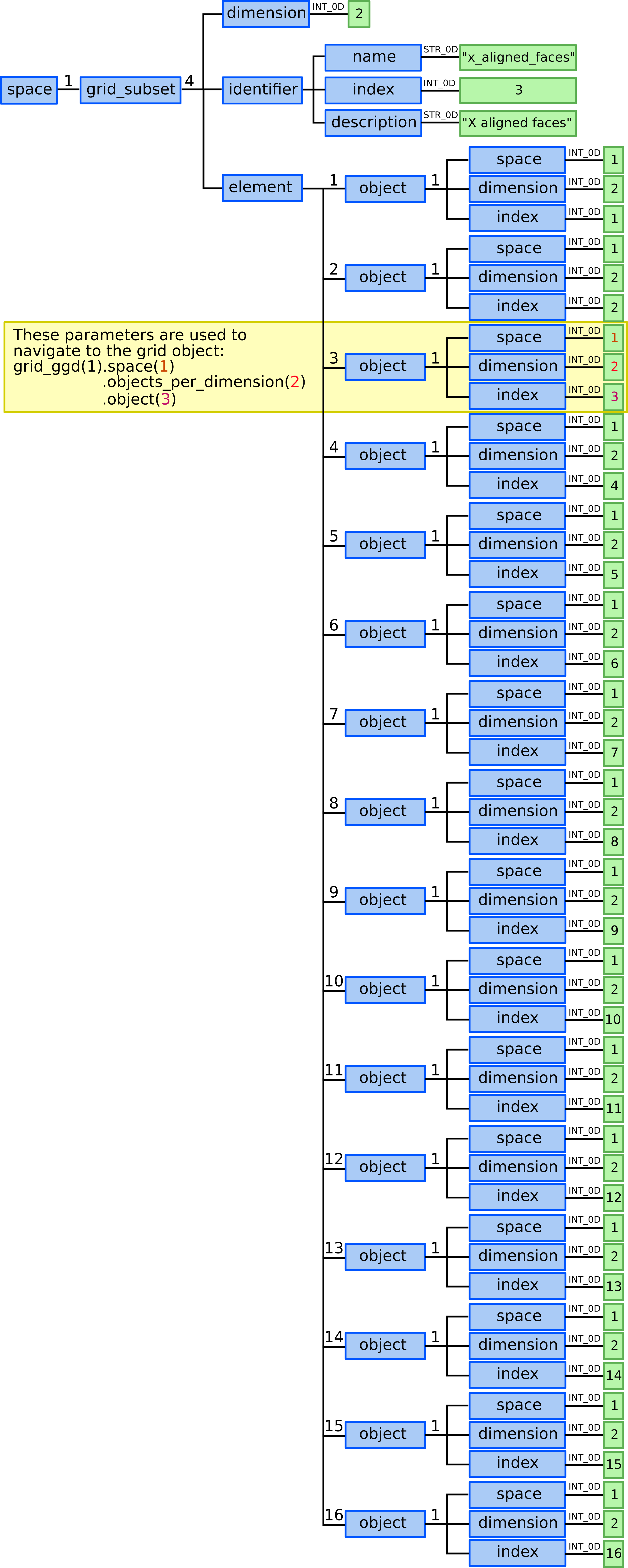
../_images/example_3_6.png — Defining the **x_aligned_faces** grid subset in GGD.¶

12.4) Define y_alignes_faces grid subset. Here we need to define 15 elements each composed by single 1D object - face.

grid_ggd(1).grid_subset(5).dimension = 2
grid_ggd(1).grid_subset(5).identifier.name = "y_aligned_faces"
grid_ggd(1).grid_subset(5).identifier.index = 4
grid_ggd(1).grid_subset(5).identifier.description = "Y aligned faces"
grid_ggd(1).grid_subset(5).element(1).object(1).space = 1
grid_ggd(1).grid_subset(5).element(1).object(1).dimension = 2
grid_ggd(1).grid_subset(5).element(1).object(1).index = 17
grid_ggd(1).grid_subset(5).element(2).object(1).space = 1
grid_ggd(1).grid_subset(5).element(2).object(1).dimension = 2
grid_ggd(1).grid_subset(5).element(2).object(1).index = 18

grid_ggd(1).grid_subset(5).element(3).object(1).index = 19
grid_ggd(1).grid_subset(5).element(4).object(1).index = 20
grid_ggd(1).grid_subset(5).element(5).object(1).index = 21
grid_ggd(1).grid_subset(5).element(6).object(1).index = 22
grid_ggd(1).grid_subset(5).element(7).object(1).index = 23
grid_ggd(1).grid_subset(5).element(8).object(1).index = 24
grid_ggd(1).grid_subset(5).element(9).object(1).index = 25
grid_ggd(1).grid_subset(5).element(10).object(1).index = 26
grid_ggd(1).grid_subset(5).element(11).object(1).index = 27
grid_ggd(1).grid_subset(5).element(12).object(1).index = 28
grid_ggd(1).grid_subset(5).element(13).object(1).index = 29
grid_ggd(1).grid_subset(5).element(14).object(1).index = 30
grid_ggd(1).grid_subset(5).element(15).object(1).index = 31

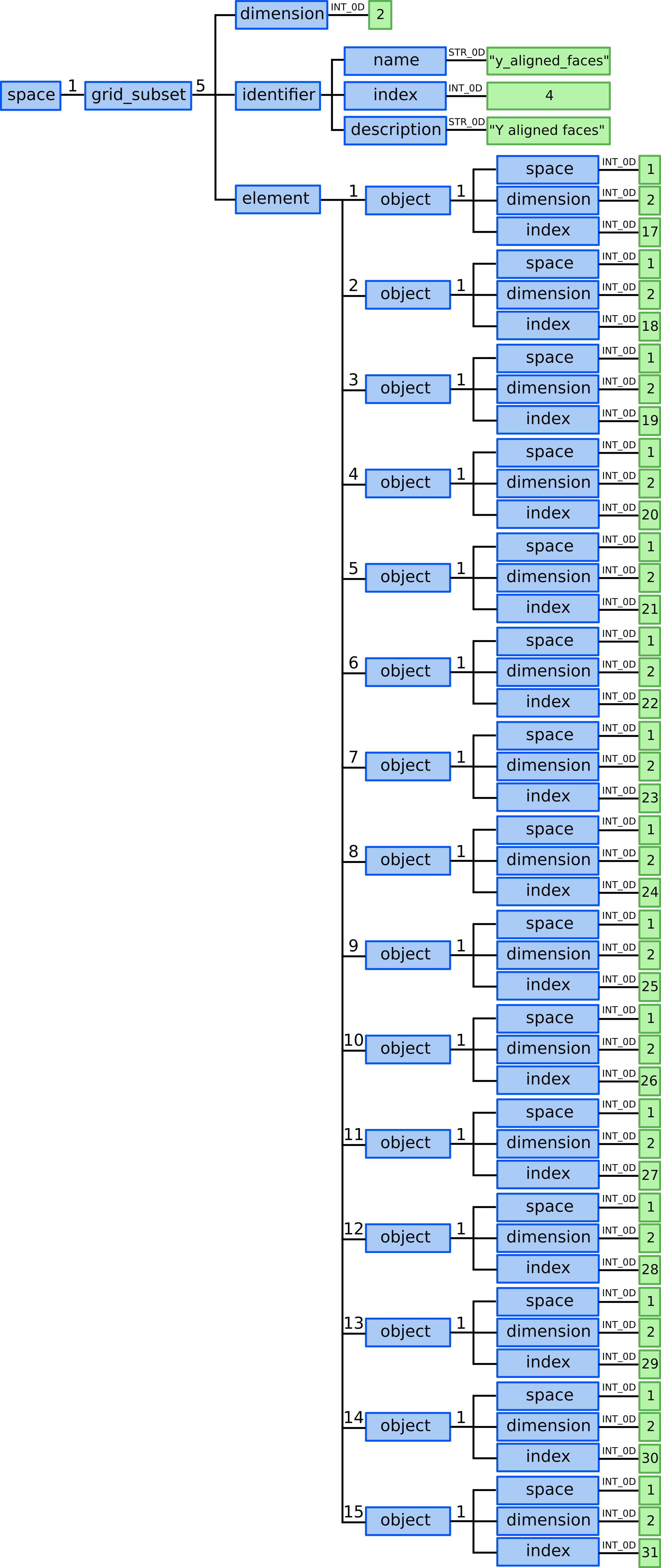
../_images/example_3_7.png — Defining the **y_aligned_faces** grid subset in GGD.¶

12.5) Define our “outer_divertor” grid subset. Here we need to define 12 elements each composed by single 2D object - cell/quad.

grid_ggd(1).grid_subset(6).dimension = 3
grid_ggd(1).grid_subset(6).identifier.name = "outer_divertor"
grid_ggd(1).grid_subset(6).identifier.index = 24
grid_ggd(1).grid_subset(6).identifier.description = "Cells defining the outer divertor region"
grid_ggd(1).grid_subset(6).element(1).object(1).space = 1
grid_ggd(1).grid_subset(6).element(1).object(1).dimension = 2
grid_ggd(1).grid_subset(6).element(1).object(1).index = 1
grid_ggd(1).grid_subset(6).element(2).object(1).space = 1
grid_ggd(1).grid_subset(6).element(2).object(1).dimension = 2
grid_ggd(1).grid_subset(6).element(2).object(1).index = 2
grid_ggd(1).grid_subset(6).element(2).object(1).space = 1
grid_ggd(1).grid_subset(6).element(2).object(1).dimension = 2
grid_ggd(1).grid_subset(6).element(3).object(1).index = 3
grid_ggd(1).grid_subset(6).element(2).object(1).space = 1
grid_ggd(1).grid_subset(6).element(2).object(1).dimension = 2
grid_ggd(1).grid_subset(6).element(4).object(1).index = 4

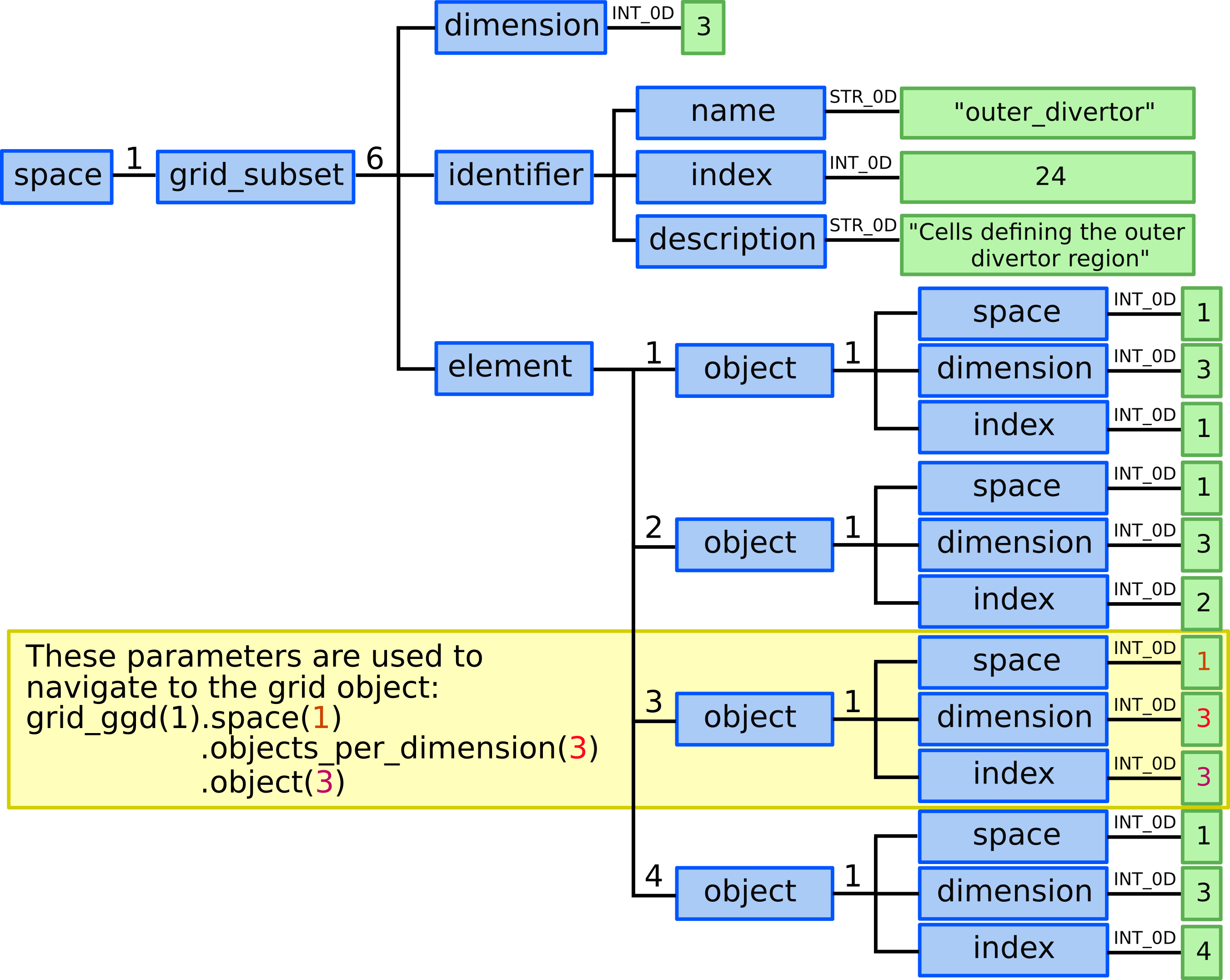
../_images/example_3_8.png — Defining the **outer_divertor** grid subset in GGD.¶

Defining physical quantities¶

In this example we assume that we have electron temperature quantities/values for two time slices (the grid is static) at times 1.0ms and 2.0ms that correlate to our 20 points and 12 quads. Defining them in GGD is done in the next way:

13.) We need to allocate two ggd AOS (two time slices).

14.) We specify time value for both time slices:

ggd(1).time = 1.0
ggd(2).time = 2.0

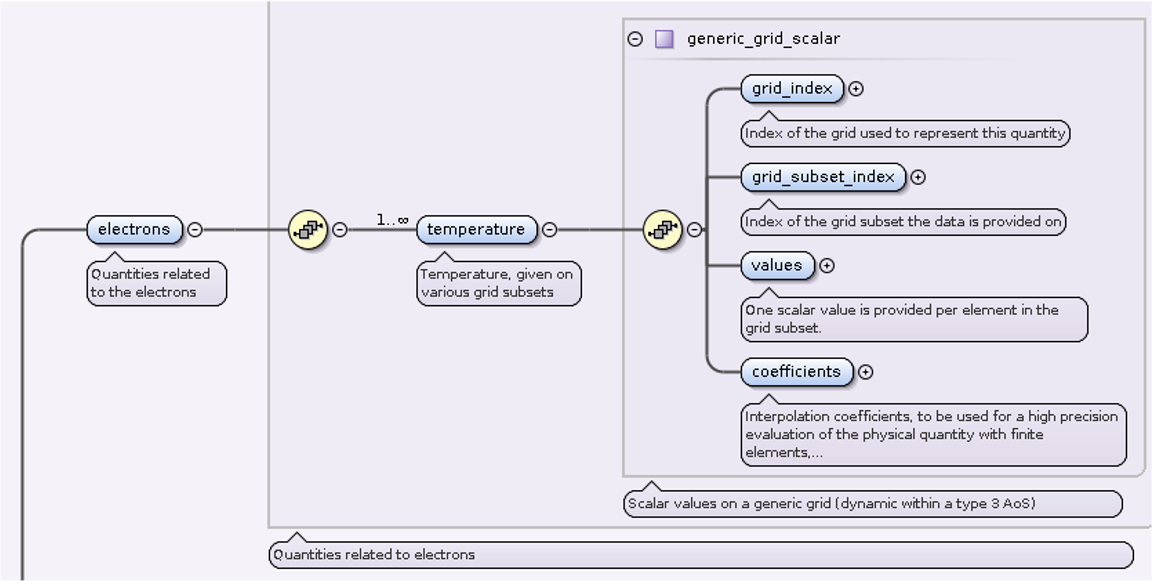
Electron temperature¶

15.) We allocate three ggd(1).electrons.temperature AOSs as in this case we have available (we assume) electron temperature quantities for three grid subsets - nodes, cells and outer_divertor.

First time slice¶

16.) In ggd(1).electrons.temperature(1) we define grid_index, grid_subset_index and values leafs.

ggd(1).electrons.temperature(1).grid_index = 1
ggd(1).electrons.temperature(1).grid_subset_index = 1
ggd(1).electrons.temperature(1).values = e.g. [1.1, 2.2, …, 20.20] (one value per point, 20 values)

17.) In ggd(1).electrons.temperature(2) we define grid_index, grid_subset_index and values leafs.

In this case it would navigate to our cells grid subset.

ggd(1).electrons.temperature(2).grid_index = 1
ggd(1).electrons.temperature(2).grid_subset_index = 5
ggd(1).electrons.temperature(2).values = e.g. [1.1, 2.2, …, 12.12] (one value per quad, 12 values)

18.) In ggd(1).electrons.temperature(3) we define grid_index, grid_subset_index and values leafs.

In this case it would navigate to our outer_divertor grid subset.

ggd(1).electrons.temperature(3).grid_index = 1
ggd(1).electrons.temperature(3).grid_subset_index = 24
ggd(1).electrons.temperature(3).values = e.g. [3.3, 4.4, 7.7, 8.8] (one value per quad, 4 values)

Second time slice¶

19.) In ggd(2).electrons.temperature(1) we define grid_index, grid_subset_index and values leafs.

In this case it would navigate to our nodes grid subset.

ggd(2).electrons.temperature(1).grid_index = 1
ggd(2).electrons.temperature(1).grid_subset_index = 1
ggd(2).electrons.temperature(1).values = e.g. [2.2, 3.3, …, 21.21] (one value per point, 20 values)

20.) In ggd(2).electrons.temperature(2) we define grid_index, grid_subset_index and values leafs.

In this case it would navigate to our cells grid subset.

ggd(2).electrons.temperature(2).grid_index = 1
ggd(2).electrons.temperature(2).grid_subset_index = 5
ggd(2).electrons.temperature(2).values = e.g. [2.2, 3.3, …, 13.13] (one value per quad, 12 values)

21.) In ggd(2).electrons.temperature(3) we define grid_index, grid_subset_index and values leafs.

In this case it would navigate to our outer_divertor grid subset.

ggd(2).electrons.temperature(3).grid_index = 1
ggd(2).electrons.temperature(3).grid_subset_index = 24
ggd(2).electrons.temperature(3).values = e.g. [4.4, 5.5, 8.8, 9.9] (one value per quad, 4 values)

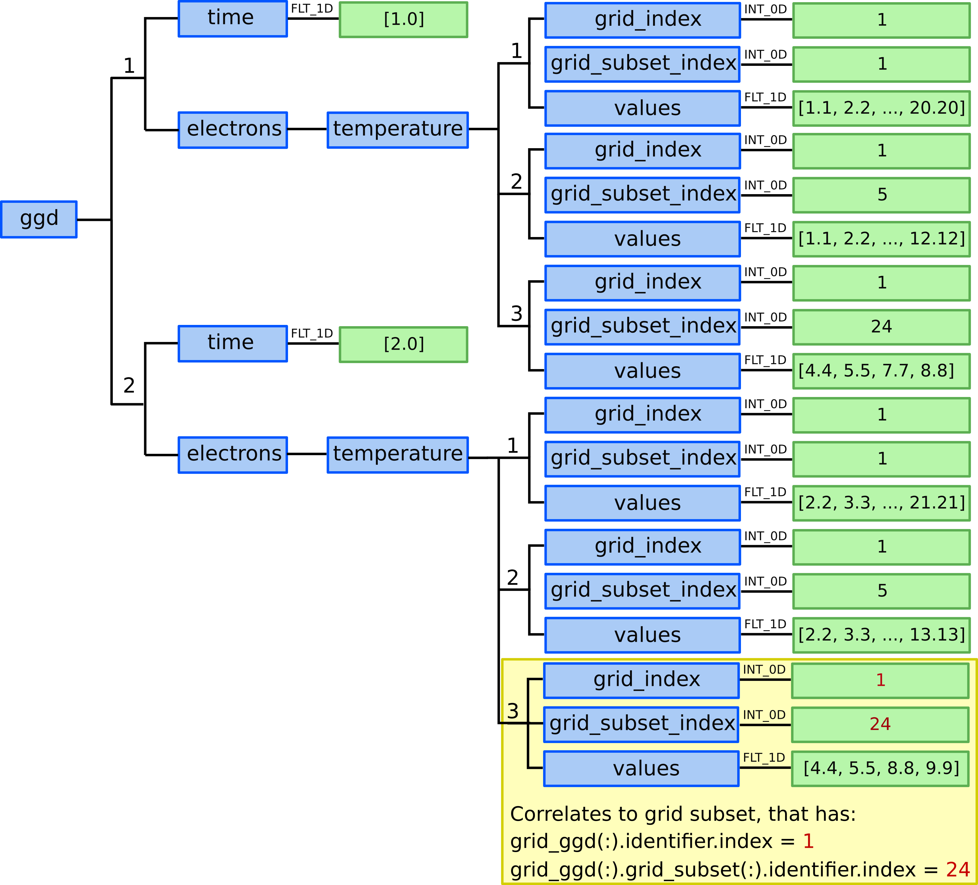
../_images/example_3_9.png — Defining electron temperature data fields for **two time slices** and **three grid subsets** - **nodes**, **cells**, and our **outer_divertor**.¶

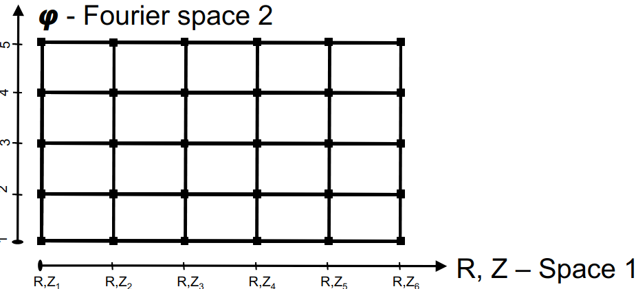
MHD example: Combined unstructured and Fourier space¶

The following example is based on the [JOREK] non-linear MHD code. JOREK uses Bezier FEM description in poloidal plane and Fourier interpolation in toroidal direction. So far, the implementaion of such geometry has not been treated in similar codes. The example follows jorek/util/IMAS/JOREK2IDS/jorekjorekHDF5toIDS.py python script that reads jorek HDF5 files and writes IDS. The most important properties that are stored are 2D grid, it’s properties and values.

The discretization of JOREK is well described in the paper [Czarny-Huysmans-2008].

For all variables indexed by \(\nu=1\dots N_{var}\) the distibution \(X(s,t,\varphi)\) of quantity \(X\) at the toroidal position \(\varphi\) in a given finite element can be expressed by

\[\begin{split}X_\nu(s,t,\varphi) =\sum_{k=1}^{N_{vert}}\sum_{j=1}^{N_{ord}}\sum_{l=1}^{N_{tor}}~ &\texttt{nodes(i).values(l,j,}\nu\texttt{)} \cdot\texttt{H}(k,j;s,t)\\ &\cdot\texttt{element.size(k,j)} \cdot Z_l(\varphi),\end{split}\]

where i=element.vertex(k) is the global node index corresponding to the vertex k of the finite element. Here, \(N_{var}\) denotes the number of physical variables, \(s\) and \(t\) are the poloidal local coordinates, H are Bezier basis functions (polynomials), element.size are geometrical coefficients for the element, \(N_{vert}=4\) the number of vertices in each element, \(N_{ord}=4\) the number of degrees of freedom per vertex, and \(N_{tor}\) the number of different toroidal Fourier modes. The quantity \(Z_l(\varphi)\) corresponds to the value of the \(l\)-th Fourier mode at the toroidal position \(\varphi\). The table below lists which Fourier modes correspond to the different mode indices \(l\) with \(n_p\) as peridicity of tyhe simulation

\(l\)	1	2	3	4	5	…
\(Z_l(\varphi)\)	1	\(\cos(n_p\varphi_p)\)	\(\sin(n_p\varphi_p)\)	\(\cos(2n_p\varphi)\)	\(\sin(2n_p\varphi)\)	…

Fourier Periodicity - \(n_p\)¶

Type of space geometry (grid_ggd.space.geometry_type)

0: standard,
1:Fourier,
>1: Fourier with periodicity

Defining the grid¶

Note

If possible, we should always decompose the discretisation into spaces: independent discretisation of individual directions.

Following above rule and JOREK discretisation there are two grid_ggd spaces:

Space 1 is two-dimensional (R,Z) space of unstructured grid with geometry_2d associated to nodes and cells. Note that the R, Z coordinates are expressed as every other quantity \(X(s,t,\varphi)\). For tokamak applications, the (R,Z) grid does not vary toroidally and only the n=0 harmonic is employed. In this case and using JOREK notation, R and Z are expressed as

\(R(s,t) =\sum_{k=1}^{N_{vert}}\sum_{j=1}^{N_{ord}}\texttt{nodes(i).x(j,1)} \cdot\texttt{H}(k,j;s,t) \cdot\texttt{element.size(k,j)}\) \(Z(s,t) =\sum_{k=1}^{N_{vert}}\sum_{j=1}^{N_{ord}}\texttt{nodes(i).x(j,2)} \cdot\texttt{H}(k,j;s,t) \cdot\texttt{element.size(k,j)}\)
1. The geometrical coefficients representing the grid (x) are stored as objects_per_dimension[0].object[i].geometry_2d(j,:)=nodes(i).x(j,:)
2. And the elements sizes \(1, d_{uk}, d_{vk}, d_{uv}d_{vk}\) under objects_per_dimension[2].object[i_elm].geometry_2d(:,:)=element.size(:,:)
Space 2 is one-dimensional Fourier space with \(\varphi\) and geometry_type.index >= 1 (Fourier) with geometry objects (1, 2, 3, …, number of harmonics)

Firstly we write every node and every cell in grid_ggd/space/object_per_dimension. Nodes are stored under index “0”. Each node has \(R, Z\) coordinate in .../geometry with derivatives (in R and Z direction and mixed) needed for calculating control points and grid’s curvature in .../geometry_2d. Cells are written in similar manner with their connectivity in geometry and 2D array size in geometry_2d. Size describes distances from nodes to cell’s control points which is also necessary for plotting more precise grid. Both size and derivatives are explained in detail in thesis by Daan Van Vugt [VanVugt19].

Defining physical quantities¶

For each physical quantity (temperature, psi, j..) values and it’s derivatives must be stored for each node. Values are in grid/variable/values

Values (Te, n, w, …), stored under GGD, with the above two spaces form a “structured” (implicitly defined) grid of node values, where explicitly RZ values of first harmonics are saved first, then RZ values of the second harmonics follow up to the last RZ harmonics. Similarly, coefficients on the nodes are saved. This definition follows column major (FORTRAN) notation, meaning that with varying first index (R) the values are close together in the memory and that the last index (\(\varphi\) in Fourier space) defines RZ block of values in memory. At the moment, the correspondance between \(X(s,t,\varphi)\) and GGD is, for example for the toroidal current density

mhd_ids.ggd[islice].j_tor[0].coefficients[l,m(i,j) ]=nodes(i).values(l,j,index_jtor)

and m(i,j)=i+(j-1)N_dof.

Bezier elements in VTK¶

Bezier geometry is the most complex, but it enables us to increase nonlinear subdivision level for same number of points within visualisation platform (such as paraview), because it uses Bezier polynomials to interpolate more points from initial control points. Calculation of control points in RZ plane used here is explained in thesis [VanVugt19].

For 2D these control points are used to create Bezier quadrilaterals. As a result each cell is made of 4×4 nodes. When we move to 3D, Bezier hexahedrons are made of 3 planes of 4×4 points, which gives us 48 nodes per cell. Because our cell is not 4x4x4 we just skip nodes that are not there. Anisotropic structure of cell’s shape is specified by SetHigherOrderDegrees() with shape[3,3,2] in jorek/utils/jorek_read_h5.py. (Even though cells are made of 4x4x3 points, one number less must be given for each dimension.)

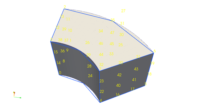
Therefore, we have anisotropic Bezier element with:

In poloidal plane exact Bezier cubic non-rational quads
In toroidal direction an approximation between toroidal planes with rational quadratic Bezier curves.

For sake of clarity a jorek/util/IMAS/JOREK2IDS/IDS_to_VTK.py script is made to read previously written data and makes .vtu for visualisation with ParaView 5.9.1 or higher. Once again we must choose some arguments to specify what we want our plot to look like. The most important are “number of planes” and \(\varphi\). Script writes object with Bezier cells if not decided differently. If Bezier is disabled the plane quadrilateral mesh (2D) without Fourier harmonics is used. However, node numbering in this case corresponds to JOREK node and cell numbering (without subdivision).